Interpretability Blog

In a previous blog post, I discussed the three main properties which make a statistical model an (intrinsically) “interpretable” model. In this blog post, I want to talk about the other side of the interpretability-explainability divide, and discuss the methods used for post-hoc explanation of generic blackbox models.

To begin, we start by recalling the modern distinction between “Interpretability” and “Explainability” as described in [1]. A model is interpretable when it is ‘intrinsically interpretable’ or it is ‘interpretable by design’. The key criteria which researchers agree make a statistical model interpretable by design were discussed at length in the previous blog post. On the other hand, a method is an explanation to a blackbox model whenever it gives a simplified interpretation or post-hoc justification to explain the reasoning process of the blackbox model. The approaches used to do this are what we will focus on in this blog post.

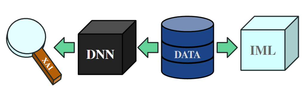
Because explainability refers to post-hoc explanations provided to an arbitrary blackbox model, there is a need to be quite flexible in what constitutes an explanation. That same flexibility is born out with the wide collection of XAI methods used throughout the literature. Nevertheless, there are also parallels between an explainability method and the interpretable model they are mimicking. Accordingly, we begin by reviewing the three major interpretability types and discuss how many XAI methods are representative of those interpretability types.

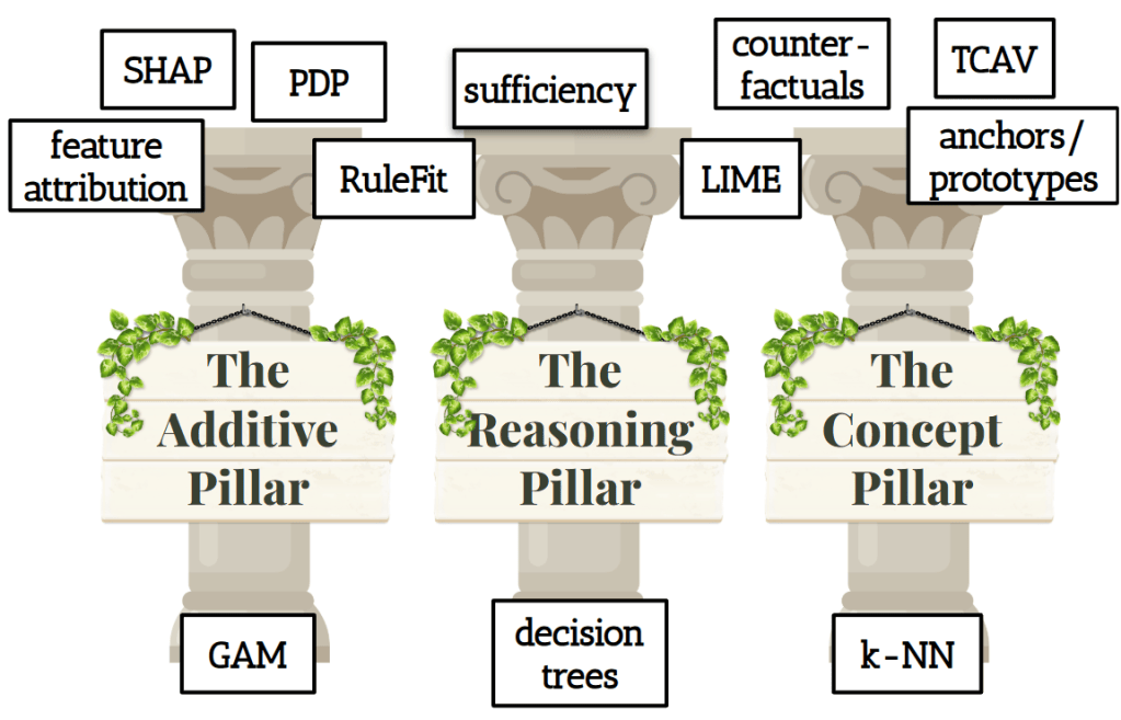
The Three Pillars of Interpretability

Last time, we went into some detail on the three major styles of interpretability based on three of the simplest reasoning methodologies: additive reasoning, logical reasoning, and concept-based reasoning. These each correspond to the simple machine learning models of: the linear model, the decision tree model, and the k-nearest neighbor model. Last time, we also discussed the basics of how they generalize in a ‘bottom-up’ sense to become the wider class of interpretable: generalized additive models, decision circuits, and concept bottleneck models. This time, we discuss the ‘top-down’ ways in which XAI methods compress arbitrary blackbox models into simplified explanations which give partial insight into their behavior.

Feature Attribution (Additive)

We begin with the most popular method of explainability: feature attribution. Whether it is the older style of gradient saliency, the newer style of model-agnostic explanation, or any other style of feature attribution, this is the type of method with the by far greatest amount of research dedication.

Starting with simple gradient saliency [2] to show which input pixels were leading to a classification decision, this research area saw several years of research, culminating in methods like SmoothGrad [3] and Integrated Gradients [4], but ultimately culminated in the negative results of ‘sanity checks for saliency maps’ [5]. There, it was pointed out how the saliency maps are not obviously more informative than something like an edge detector, and that moreover randomization studies showed that much of the informativeness of saliency explanations appeared equally valid when run on a randomly initialized CNN.

SHAP [6] picked up around this time and worked on the model-agnostic formulation which was increasing in popularity at the time, rather than putting requirements on the blackbox model like differentiability. This method has become the most-used explainability method with ongoing debates over its interpretation, its implementation details, and its best use cases. It has even inspired its own set of extensions to interaction values [7] in a way which the original game theory literature of Shapley values [8] had never discovered. Beyond its incredible popularity and its active research, it even connects to older attribution-like explainability methods like PDP (partial dependence plots) [9] which plots the average effect of changing an individual feature. Unfortunately, this story does not necessarily have a happy ending, and this connection between SHAP and PDP makes clear the connection with GAM models [10], meaning the SHAP approach and all other feature attribution approaches share some of the same fundamental limitations, namely: their inability to represent feature interactions. Although interaction attributions extending SHAP [7] or otherwise patch up this limitation, it remains the fundamental shortcoming of additive-style methods of feature attribution. Accordingly, let us look towards other completely different styles of explanation to round out our understanding of explainability.

Feature Sufficiency (Logical)

A second type of feature-based explanation which has not received as much research attention as the attribution style approaches is the methods of feature sufficiency. Rather than attribution which asks how much a feature (additively) contributed to a final prediction, sufficiency is instead inspired by boolean circuits and asks whether or not a feature was necessary and/or sufficient for the prediction. Conversion to continuous features is commonly done by adding a small epsilon ball around the current feature value (similar to adversarial learning) and conversion to continuous outputs is commonly done by adding a small epsilon tolerance around the predicted value.

The most pure of these types of methods are sufficient input sets [11] and necessary input sets [12], which ask which subset of the features are sufficient to keep the same prediction and which subset of the features are necessary to keep the same prediction. Both are generally interested in the minimal subsets which achieve this, both in the global minimal sense (cardinality) and in the local minimal sense (no strict subsets). Works like [13] extend these local explanations to a more global explanation by providing a complete collection of sufficient input sets, providing efficient algorithms for these explanations if they are already converted into an (interpretable) boolean circuit. These approaches also have an interesting connection to counterfactual explanations [12] which we will explore further in the next section.

Interestingly, these explanation methods working directly with logical explanations actually postdate the earliest approaches incorporating logical rules. RuleFit [14] learns sparse linear combinations of logical rules from short decision trees to provide an interpretable approximation of a complex, uninterpretable decision forest. In this way, RuleFit combines both logical simplicity and additive simplicity at the same time to provide an explanation which is not as difficult to understand. Anchors [15] finds a logical rule which is sufficient to keep a prediction, but instead of only choosing a subset of inputs which are sufficient to keep fixed, it instead finds a logical rule obeyed by the input example which is sufficient to keep fixed. This is also similar in some sense to how LIME [16] finds a subset of the input space which is then fits a small interpretable model, either a sparse linear model (additive) or a small decision tree (logical). We discuss the connections between local counterfactuals and regional explanations in the next section. Although there are very few papers making this explicit [17], feature sufficiency methods also have fundamental limitations in the behavior they can easily explain.

Learned Features (Concepts)

As always, the techniques connected to concept-based interpretability are the most varied and free-form. Accordingly, we divide this section into first discussing the region-based explanations with the most straightforward connections to k-NN and prototype methods before then discussing the explainability methods connected to the broader sense of concepts found in concept bottleneck models.

Starting by picking up the conversation from the last section on Anchors [15] and LIME [16], let us remind ourselves that LIME first picks a small region around the input example and then tries to fit an interpretable model which is accurate, at least in this small region. Taking, for instance, the linear explanation and taking the region size to zero, we are essentially recovering the definition of the gradient. We could easily come up with a gradient-like definition for the decision tree. This helps to make clear how the goal of LIME is to balance between the complexity coming from the global, semi-global, or local explanation and the complexity coming from the interpretable model (additive or logical). Anchors instead tries to cover a larger region through the use of a logical rule, rather than a distance-based alternative. It is for this reason, we can see that both approaches are a type of counterfactual explanation [18], but one is a counterfactual in the logical sense of alternative feature values [12], whereas the classical counterfactual explanation instead focuses on closeness as described by a predefined distance metric [18]. The prototype method and k-NN method are defined in this sense of distance comparisons, rather than the logical sense of feature values being the same i.e. Hamming distance. Another explainability approach using this distance-based style of explanation is the method combining prototypes and criticisms together [19]. Here, not only positively attracting examples of the correct class are included, but also the examples which are poorly represented by the prototypes are listed as criticisms.

Beyond assuming a fixed distance metric, there are also methods building their own distance metrics (usually implicitly) through self-defined regions or concepts. A major approach here are the regional explanations combining feature attribution with self-discovered local regions [20, 21]. These works attempt to explicitly balance the additive complexity of minimizing feature interactions with the regional complexity of minimizing the number of regions. Works attempting to use human-defined concepts like TCAV [22] take a dataset of human-labeled concepts and attempt to extract the neural network representations which are corresponding to the human concepts.

Mechanistic Explanations

A fourth approach to explainability which does not neatly fit into any of the above three categories is the field of mechanistic interpretability. (Yes, mechanistic interpretability is technically explainability; no, I don’t think we should rename it.) Although many of its methods clearly fall into the category of concept-based interpretability, with linear probes and nonlinear probes being souped up versions of TCAV, and with feature visualization and sparse autoencoders being equivalent version for machine-defined concepts in place of human-defined concepts, many other methods do not easily fall into this category. The discovery of sparse circuits [23] and causal graphs [24] is much closer to a logic-based interpretability trying to discovering the underlying circuit mechanics of the models’ computation. Additionally, basic tools of feature attribution like gradient saliency, SHAP, and other attribution methods are commonly used for their generic applicability.

In some sense, mechanistic interpretability is even more ‘top-down’ than all of the top-down methods of more classical explainability. This seems to be inspired in part by the focus on the tasks of CV and NLP (with CNNs and LLMs) which foreground the blackbox model as the highest priority. Where interpretability methods, especially on tabular data, are willing to sacrifice model complexity for minor drops in accuracy, the same cannot be done in the fields of CV and NLP (which are the fields which fueled the deep learning revolution in the first place).

Although each individual method usually falls quite squarely into one of the above three categories, I still find it worthwhile to separate out mechanistic interpretability into its own section. That is because it has managed not only to separate itself culturally from interpretability research, but thereby finds itself less concerned with the validity of its explanations so long as they make progress towards the grand goal of understanding the LLM in its entirety.

The Duality of Interpretability and Explainability

It is my belief, coming from the interpretability side of things, that all of these explanation methods will ultimately face the same fundamental tradeoffs as seen in feature attribution and feature sufficiency. There will be an increasing number of theoretical results showing the duality between interpretable model A and explainability method B to the point where we very clearly understand the boundaries between these approaches, and further understand the fundamental limitations in explanations applied to blackbox models. For SHAP and feature attribution, this limitation is the GAM (with interaction complexity). For sufficiency and necessity, this limitation is the decision circuit (with query complexity). Although concept-based methods are designed to be sufficiently general, prototype-based approaches already have some clear limitations in their explanatory power.

In the long run, the existing dualities [10, 17] will be joined by an increasing library of correspondences between interpretability methods and explainability methods to the point where explainability method B can be understood as an A-based interpretable approximation of a given blackbox model. In such a world, it will become clear that no interpretability/explainability method will be strictly more powerful than another and that each target application will require the appropriate interpretability tool, and that moreover, combinations which balance the usage of each of these different styles of interpretability, especially amongst the major three pillars, will be the most effective at providing interpretability to previously incomprehensible models.

For these reasons, classical interpretability is now the champion of the subfield of interpretability and mechanistic interpretability is now the champion of the subfield of explainability. Continued progress, both theoretical and empirical, will hopefully continue to narrow the gap between the approaches and come to shared conclusions on which methodologies are appropriate under what scenarios. Interpretability should continue to build up the available toolkit of practical models which we trust as glassbox models and understand the fundamental limitations of these approaches. Explainability should continue to chip away at the complexity of the most important blackbox models of our time -CNNs, diffusion models, and LLMs – in hopes of making steps towards a greater fundamental understanding of the algorithms, concepts, features, etc. used by those blackbox models. Both are necessary to make progress on the challenging and fundamental question of how to achieve interpretability.

[1] Rudin, Cynthia. (2019). “Stop explaining black box machine learning models for high stakes decisions and use interpretable models instead”.

[2] Simonyan, Karen et al. (2014). “Deep Inside Convolutional Networks: Visualising Image Classification Models and Saliency Maps”

[3] Smilkov, Daniel et al. (2017). “SmoothGrad: removing noise by adding noise”

[4] Sundararajan, Mukund et al. (2017). “Axiomatic Attribution for Deep Networks”

[5] Adebayo, Julius et al. (2018). “Sanity Checks for Saliency Maps”

[6] Lundberg, Scott and Lee, Su-In (2017). “A Unified Approach to Interpreting Model Predictions”

[7] Muschalik, Maximilian et al. (2024). “shapiq: Shapley Interactions for Machine Learning”

[8] Shapley, Lloyd. (1953). “A value for n-person games”

[9] Friedman, Jerome. (2001). “Greedy function approximation: A gradient boosting machine”

[10] Bordt, Sebastian and von Luxburg, Ulrike. (2023). “From Shapley Values to Generalized Additive Models and Back”

[11] Carter, Brandon et al. (2019). “What made you do this? Understanding black-box decisions with sufficient input subsets”

[12] Mothilal, Ramaravind Kommiya et al. (2021). “Towards Unifying Feature Attribution and Counterfactual Explanations: Different Means to the Same End”

[13] Darwiche, Adnan and Hirth, Auguste. (2020). “On The Reasons Behind Decisions”

[14] Friedman, Jerome and Popescu, Bogdan. (2008). “Predictive learning via rule ensembles”

[15] Ribeiro, Marco Tulio et al. (2018). “Anchors: High-Precision Model-Agnostic Explanations”

[16] Ribeiro, Marco Tulio et al. (2016). “Why Should I Trust You?: Explaining the Predictions of Any Classifier”

[17] Günther, Eric et al. (2025). “Informative Post-Hoc Explanations Only Exist for Simple Functions”

[18] Wachter, Sandra et al. (2018). “Counterfactual Explanations without Opening the Black Box: Automated Decisions and the GDPR”

[19] Kim, Been et al. (2016). “Examples are not enough, learn to criticize! criticism for interpretability”

[20] Herbinger, Julia et al. (2022). “REPID: Regional Effect Plots with implicit Interaction Detection”

[21] Herbinger, Julia et al. (2024). “GADGET: Decomposing Global Feature Effects Based on Feature Interactions”

[22] Kim, Been et al. (2018). “Interpretability Beyond Feature Attribution: Quantitative Testing with Concept Activation Vectors (TCAV)”

[23] Marks, Samuel et al. (2025). “Sparse Feature Circuits: Discovering and Editing Interpretable Causal Graphs in Language Models”

[24] Geiger, Atticus et al. (2025). “Causal Abstraction: A Theoretical Foundation for Mechanistic Interpretability”